The Rule of Five - Making good calls from limited data

We frequently make decisions based on imprecise information. This is true for executives who must choose between projects with different potential returns on investment and engineers who prioritize bug fixes over new features based on anticipated customer impact.
Data is necessary for making informed decisions. Often, we lack the time or resources to run a thorough data analysis. Usually what happens is that we rely primarily on intuition. After all, we’re experts in our fields, right? We should be able to make educated guesses mostly based on experience.
However, humans tend to be biased toward overconfidence. It’s a well-established bias, known as the overconfidence effect. Do you remember the last time (or ever) you finished a large project on time without having to “power through” and work late nights?
This article presents a simple yet effective technique to fight this natural bias for making reasonable estimates when faced with quick decisions and limited resources.
The Rule of Five
Imagine you want to estimate something. For example, the price your customers are willing to spend for a brand-new feature, the duration of a unit test in your test suite, or the time to fix a production issue. When asked about the statistically significant sample size, you might think you need at least 100 or even 1,000 observations.
But what if I told you that you can gain valuable insights from a mere five observations? What if you can still derive some statistically significant insights from a sample of 5 observations?
In his book “How to Measure Anything - Finding the Value of Intangibles in Business”, Douglas Hubbard presents a rule of thumb called the “Rule of Five”, which is defined as follows.
Rule of Five: There is a 93.75% chance that the median of a population is between the smallest and largest values in any random sample of five from that population.
In other words, there’s a greater than 90% probability that the true population median lies between the minimum and maximum values of five randomly selected observations.
This is a surprising claim, and after reading this I wanted to verify this myself. So let’s put the “Rule of Five” into practice and see if it holds water.
Empirical Test
We’ll use Python and the numpy library. Let’s import it:
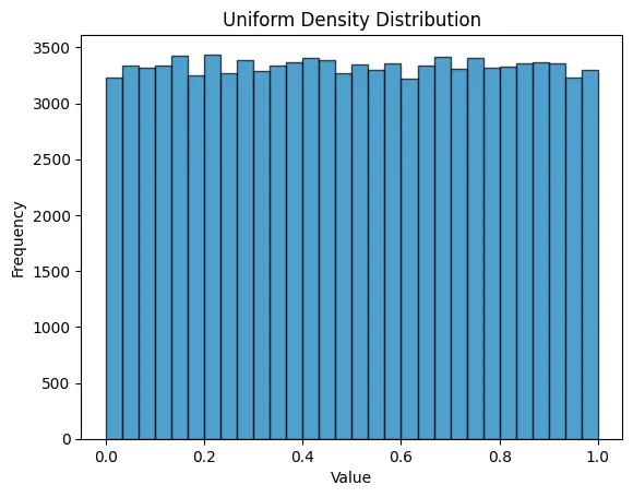
import numpy as npWe’ll start with a simple example using a uniform distribution. We’ll create a random array of 100,000 entries where each entry has an equal probability of being between 0 and 1.
# Create a new random generator with a seed to ensure reproducibility.
SEED = 122807528403841006732342137672332424409
rng = np.random.default_rng(SEED)

# Create random numbers following a uniform distribution.
POPULATION_SIZE = 100_000
uniform = rng.uniform(0, 1, POPULATION_SIZE)
Here’s the density distribution:
Now let’s define our “Rule of Five” in Python. The rule_of_five function takes as argument a population as a list[float] and return a True if the rule passes and False otherwise.
def rule_of_five(population: list[float]) -> bool:
sample = rng.choice(population, 5, replace=False)
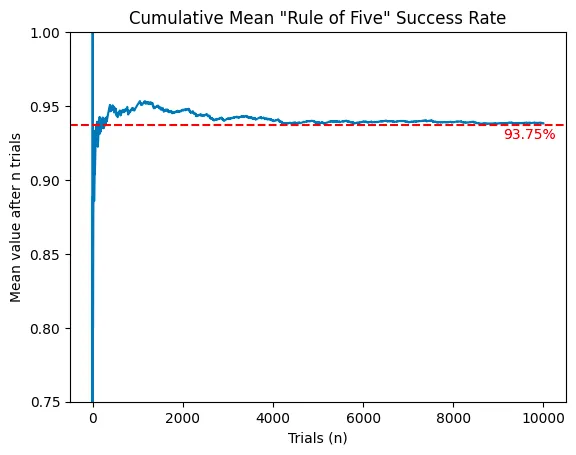
return sample.min() <= np.median(population) <= sample.max()Let’s run it 10,000 times and calculate the success rate:
TRIAL_COUNT = 10_000
rule_of_five_results = np.array([rule_of_five(uniform) for _ in range(TRIAL_COUNT)])

success_rate = rule_of_five_results.mean()
print(f"Rule of five success rate: {success_rate.mean():.2%}")
With the uniform distribution, the success rate is 93.82%, very close to the theoretical 93.75%. Plotting the cumulative success rate over trials shows it quickly converges after 4,000 tests:
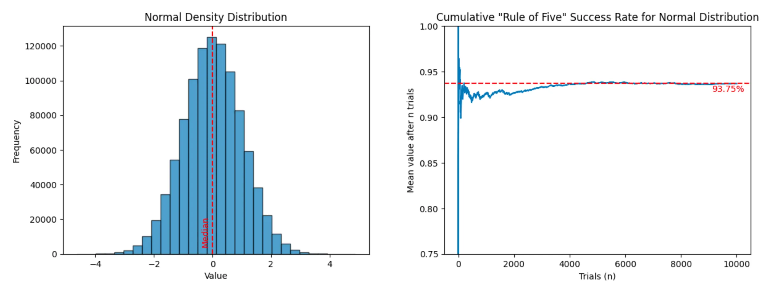
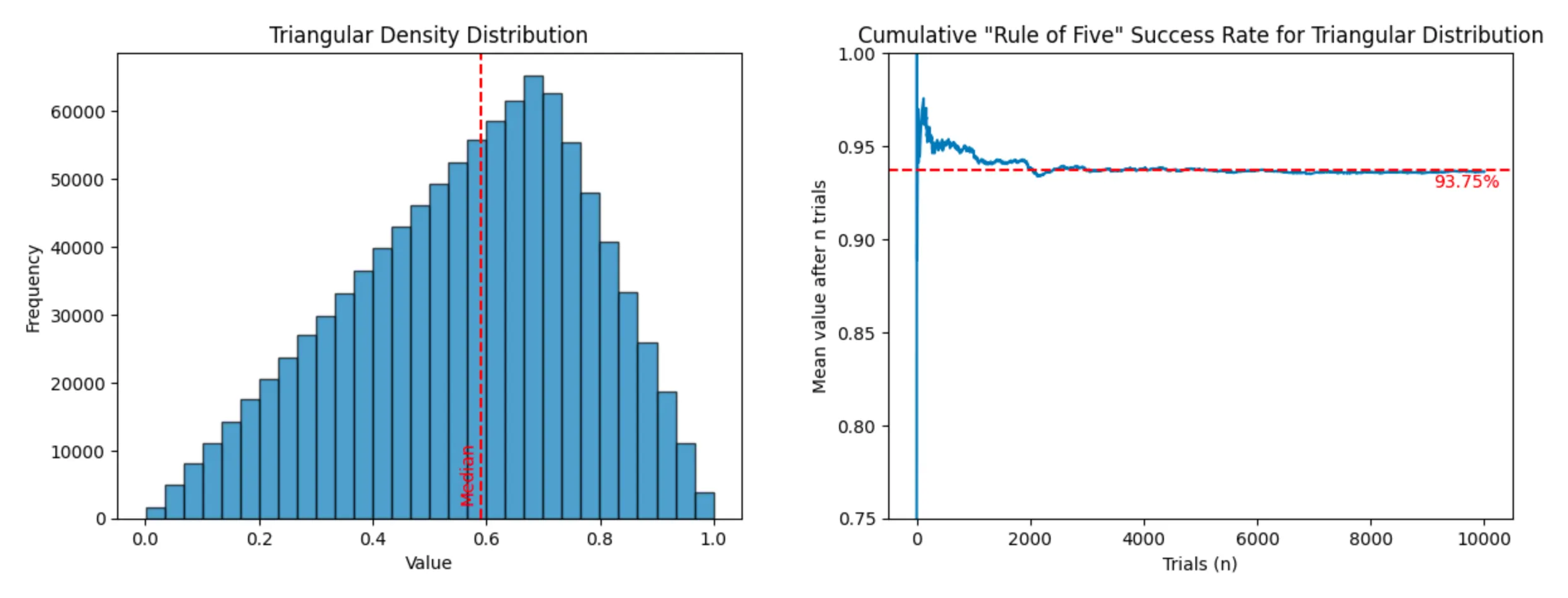
Now that we’ve seen it work with a simple uniform distribution, let’s test it against other known data distributions:
Normal distribution: (success rate: 93.68%)
Triangular distribution (success rate: 93.64%)
For those still skeptical (like me), let’s run the experiment on real-world data:
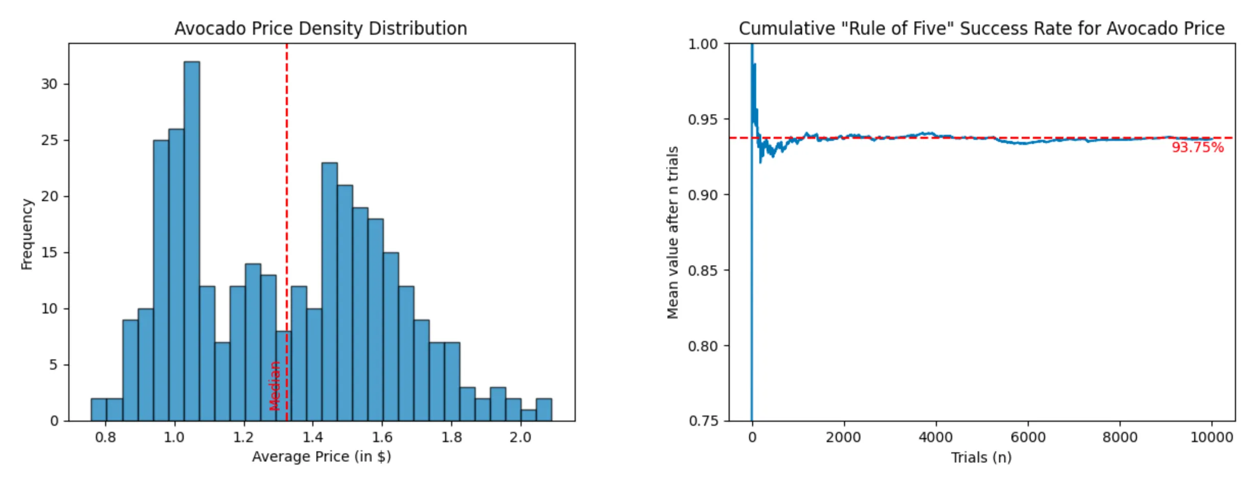
- US Avocado price between January 2015 and March 2018 (dataset - 338 entries)
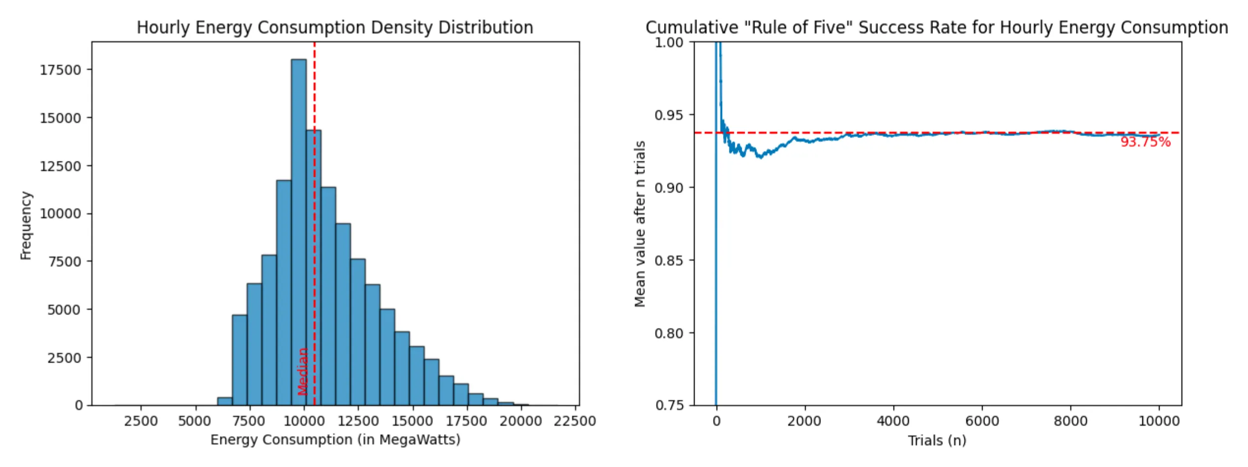
- Hourly energy consumption in the state of Virginia (dataset - 116,189 entries)
- Heart rate of a Fitbit user (dataset - 285,461 entries)
Avocado Price (success rate: 93.64%)
Energy Consumption (success rate: 93.57%)
Heart Rate (success rate: 92.71%)
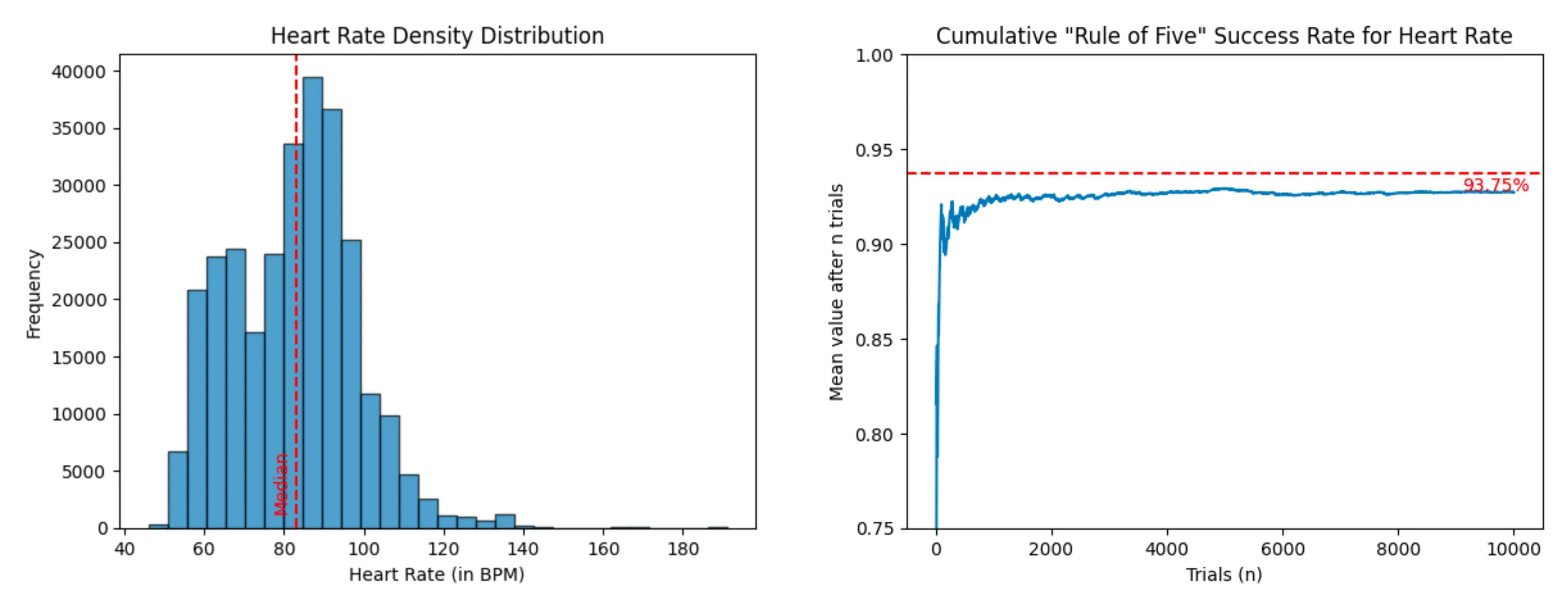
In other words, think twice the next time you consider buying an Apple Watch to monitor your median heart rate. You might be better off taking your pulse five times throughout the day. Also if you want to try it out yourself, you can find the code for the analysis at this link.
Forming a Mental Model
While it may seem counter-intuitive at first, it appears that the “Rule of Five” actually applies to any dataset, regardless of its size and distribution. It works because the “Rule of Five” is an application of Order statistics. Let me break this down for you.
With the median being the midpoint of a given dataset, there is an equal probability of picking a random value below or above the median value. Similar to flipping a coin, there is a 50/50 chance of getting heads or tails. Applying the “Rule of Five” and picking five random values above the median is like incorrectly predicting the coin side five times in a row. There is a 3.125% probability of such an event occurring:
The same reasoning can be applied to picking five random samples from the population and having all of them below the median value. There is also a 3.125% chance that all five observations are below the median.
Since “all observations are above the median” and “all observations are below the median” are mutually exclusive, the probability of the union, “all observations either are above or below the median”, is equal to the total probability of each independent event: 6.25%
This is how the “Rule of Five” can assert that there is a 93.75% chance for the population median to be within the minimum and maximum values of the five-item sample:
Conclusion
You may be wondering why the number five was chosen for the “Rule of Five” instead of four or six. I believe that Douglas Hubbard, the author of this rule, picked the number five for two reasons. First, it is a memorable number. But most importantly, it is the smallest sample size with a probability greater than 90%. When it comes to estimating something, having a 90% confidence about is usually sufficient.
| Sample Size | 2 | 3 | 4 | 5 | 6 | 7 | 8 |
|---|---|---|---|---|---|---|---|
| Probability | 50.00% | 75.00% | 87.50% | 93.75% | 96.88% | 98.44% | 99.22% |
Before concluding, something that I haven’t talked about much in this article is the sample selection. This “Rule of Five” only works when the selection samples are truly random. Don’t try to estimate the median cheese consumption per capita worldwide by surveying your French friends.
At the end of the day, the “Rule of Five” will never replace a thorough data analysis. It is simply a tool in your toolkit to quickly make informed decisions when you don’t have the complete dataset at hand or time to do a thorough analysis.
Thanks to Martin Presler-Marshall, Nolan Lawson and Kevin Venkiteswaran for the feedback on the draft of this post.